Every crude oil price you will ever trade is the market’s running estimate of one question: are there too many barrels right now, or too few? Oil supply and demand set that answer, inventories keep the score, and the futures curve publishes it in real time. Everything else – OPEC headlines, hurricane maps, EIA Wednesdays – is input. This piece builds the fundamental framework a desk analyst actually uses, and it slots into the broader toolkit in our complete guide to crude oil trading.
Fair warning on style: fundamentals are unfashionable because they are slow. But the traders who survive decades in this market are, almost without exception, the ones who can tell you the global balance to within half a million barrels a day from memory.
The Supply Side: Where 105 Million Barrels a Day Come From
Global crude and liquids production runs at roughly 105-106 million barrels per day (mb/d). Three producers dominate, and their behavior could not be more different.
- United States (~13.5 mb/d crude): The world’s largest producer, built on shale – Permian, Eagle Ford, Bakken. Thousands of independent companies responding to price, not policy. US output roughly went from 5 mb/d in 2008 to over 13 mb/d, the largest supply-side shift in modern market history, and turned the US into a major exporter after the crude export ban ended in late 2015.
- Russia (~9-10 mb/d): Conventional fields, state-influenced companies, output redirected from Europe to Asia at a discount since 2022 sanctions. Data quality: poor and worsening.
- Saudi Arabia (~9-10 mb/d): The swing producer, deliberately holding around 3 mb/d of spare capacity and producing below capability for price management.
Behind them: Canada (~5 mb/d, oil sands, growing quietly), Iraq (~4.3 mb/d), China (~4 mb/d, declining and import-hungry), UAE, Iran (sanctions wildcard), Brazil (~3 mb/d and one of the strongest non-OPEC growth stories via deepwater pre-salt), Kuwait, Mexico. The structural split that matters for analysis is not OPEC versus non-OPEC by name – it is policy barrels versus price barrels. Roughly 40 percent of world supply is managed by the OPEC+ alliance as a matter of policy; the rest shows up whenever price clears cost.
The Decline-Rate Treadmill
One supply-side fact deserves more attention than it gets: existing oil fields decline. Conventional fields lose output at mid-single-digit rates annually; shale wells lose more than half their flow in the first couple of years. Weighted across the world’s producing base, the industry must add several million barrels per day of new capacity every single year just to keep supply flat – before meeting a single barrel of demand growth. This is why “underinvestment” is a bullish thesis with a long shelf life: capital expenditure cuts made today create supply gaps two to five years out, invisible in current data. It is also why supply forecasts err in both directions – analysts extrapolate current output while the treadmill quietly accelerates underneath it. When you hear that upstream capex has fallen for consecutive years, mark your long-dated balance tighter, whatever spot inventories say.
The Demand Side: Who Burns It
Global demand runs near 103-104 mb/d. The United States remains the largest consumer at roughly 20 mb/d of petroleum products, followed by China around 16 mb/d and India near 5.5 mb/d – and India is now the fastest-growing large source of demand. Japan, South Korea and Europe are mature and flat-to-declining; the growth story for the next decade is South and Southeast Asia.
Composition matters as much as totals. Transportation fuels – gasoline, diesel, jet – account for roughly 60 percent of demand, petrochemical feedstocks a growing 15 percent or so, with heating, power and industrial uses making up the rest. That mix drives two behaviors traders must internalize. First, demand is cyclical: freight and driving track GDP tightly, so oil demand catches every macro cold. Second, demand is seasonal: summer driving season lifts gasoline pull, winter lifts heating fuels, and refinery maintenance in spring and autumn temporarily cuts crude demand regardless of what end-users are doing – refineries, not motorists, are crude oil’s actual customers. Miss that distinction and the spring inventory builds will fool you every year.
The China Problem in Every Demand Model
For two decades, the marginal barrel of demand growth has been Asian, and China’s opacity makes it the hardest input in any balance. Chinese “demand” is usually inferred: refinery runs plus net imports, adjusted for inventory change nobody can observe directly. When Beijing builds strategic or commercial stocks, imports overstate consumption; when it draws them, imports understate it. Entire quarters of apparent Chinese demand weakness have later turned out to be destocking, and vice versa. Treat Chinese import surges near price dips as opportunistic reserve building – a soft bid under the market – rather than proof of booming consumption, and hold your China numbers with looser fingers than your US ones. India, by contrast, publishes cleaner consumption data and has become the more trustworthy signal of structural Asian growth. When Chinese and Indian import trends diverge, weight the Indian number.
Refining: The Middleman That Distorts the Signal
Crude oil demand is really refinery demand, and refineries have their own economics. They buy crude when refining margins – crack spreads, the gap between product prices and crude cost – justify running, and they cut runs when margins compress, regardless of what end-consumers are doing. This middleman layer regularly confuses newcomers reading the data.
Consider what happens when gasoline demand jumps but refineries are already at full utilization: gasoline prices and crack spreads rip higher, while crude barely moves – the bottleneck is refining capacity, not crude supply. Or the reverse, a refinery outage: crude demand falls (bearish crude) while product prices spike (bullish gasoline). Same event, opposite signals, and the crude-only trader misreads both. During the 2022 diesel squeeze, distillate cracks blew out to levels several times their historical norms while crude itself traded well off its highs; the tightness lived in refining, not in the wellhead balance.
Practical implications: track refinery utilization and turnaround calendars as demand-side data; watch the 3-2-1 crack spread as a health check on real product demand; and when crude and cracks diverge, believe the cracks – products are one step closer to the end consumer.
How Oil Supply and Demand Set the Price

The mechanism is brutally simple and worth stating precisely. Production and consumption almost never match on any given day; the difference flows into or out of inventories. Prices move to whatever level forces the imbalance to correct – discouraging supply and stimulating demand when stocks are bloated, doing the reverse when stocks are scarce.
What makes oil violent is inelasticity. In the short run, a 1 percent price rise cuts demand by perhaps 0.05 percent – commuters still commute at $95 crude. Longer horizons are more forgiving (long-run elasticity estimates run near -0.3 as fleets and habits adjust), but in the window traders live in, demand barely responds. Supply is nearly as stiff: conventional fields cannot ramp quickly and hate shutting in. So a surplus or deficit of even 1 mb/d – one percent of the market – cannot be closed by gentle price moves. It gets closed by ugly ones. This is why oil regularly swings 50 percent in a year while consumption changes low single digits. Volatility is not a malfunction of the oil market; it is the direct arithmetic consequence of two nearly vertical curves intersecting.
The 2020 episode is the permanent exhibit. Pandemic lockdowns cut global demand by something on the order of 20 mb/d within weeks. No plausible price could restore that demand or shut supply fast enough; inventories absorbed the difference until storage at Cushing, Oklahoma – the delivery point for NYMEX WTI – was effectively spoken for. On 20 April 2020, longs in the expiring May WTI contract, facing physical delivery with nowhere to put the barrels, paid to get out: the contract settled at minus $37.63. Supply and demand did not just set the price; they set it below zero.
Demand Destruction: The Ceiling No One Announces
Elasticity is small, not zero, and it grows with time and pain. Sustained high prices eventually destroy demand – not smoothly, but in behavioral steps: carpooling and trip-chaining first, then airline schedule cuts, then industrial fuel switching, then recession doing the rest. In 2008, US gasoline demand was already falling year-over-year months before the financial crisis hit, with crude in the $120-140 range. In 2022, $5 US pump prices produced measurable demand declines within weeks. The signals to watch are product-side: weekly implied gasoline demand rolling over versus seasonal norms, jet fuel bookings, diesel consumption diverging from freight indices. Demand destruction is the market’s automatic stabilizer, and spotting it early is one of the few edges available to a patient fundamental trader, because headline writers are always months behind the gasoline data.
Policy Barrels: OPEC+ Quotas and Spare Capacity
The single largest recurring influence on the supply side is deliberate: OPEC+ manages roughly 40 percent of world production through negotiated quotas, and in recent years has held back several million barrels per day of capacity – group-wide cuts plus additional voluntary reductions led by Saudi Arabia – to support prices. The mechanics, politics and compliance games deserve their own study, and we cover them in depth in our guide to how OPEC controls oil prices. For balance-building purposes, three facts carry most of the weight:
- Announced cuts are not delivered cuts. Compliance historically runs well short of 100 percent; discount accordingly.
- Spare capacity is the market’s shock absorber. When Saudi Arabia, the UAE and Kuwait hold 3-4 mb/d of idle capacity, supply outages get shrugged off. When spare capacity is thin, the same outage produces a violent rally. Always know the current cushion.
- Quota decisions transmit with a lag – allocations, loading programs, then inventories – so the announcement moves price weeks before it moves a single physical barrel.
Price Barrels: US Shale as the Marginal Supplier
Shale rewired the supply side’s response speed. A shale well is drilled and producing within months, front-loads most of its output into the first two years, and then declines steeply – which means the industry must keep drilling just to stand still, and drilling decisions track price almost mechanically. Rough breakeven bands: the best Permian acreage works in the $35-45 range, with other basins – Eagle Ford, Bakken, Niobrara – strung between roughly $40 and $60.
The result is a feedback loop that operates on a horizon of months, not the multi-year cycles of conventional megaprojects. Sustained WTI above the mid-$70s pulls rigs back to work and adds supply within two or three quarters; sustained prices below $50 idles rigs and lets decline rates bite. Shale is, in effect, a price-triggered swing producer that competes with OPEC’s policy-triggered one – and the interaction between the two defines the modern crude band. Watch the Baker Hughes rig count (published Fridays) and quarterly shale-company capital budgets: they are supply data wearing a three-month delay.
The Cost Curve: Who Supplies the Last Barrel
Over multi-year horizons, price gravitates toward the cost of the marginal barrel – the most expensive supply the market still needs. Stack global production from cheapest to dearest and you get the industry cost curve: Gulf OPEC conventional at the bottom (lifting costs in the single digits), Russian conventional and the best Permian acreage in the low-to-mid range, average shale and offshore in the middle, and oil sands growth projects, some deepwater and marginal shale at the top, needing roughly $60-80 to justify new investment.
Two uses for this mental model. First, it anchors long-run fair value: when price sits far above the marginal cost of the last needed barrel, investment floods in and the excess eventually corrects, as 2011-2014’s $100-plus plateau did; when price sits below it, decline quietly wins and the market tightens, as 2015-2017 showed. Second, it explains why the marginal producer keeps changing – shale’s cost deflation in the 2010s dragged the whole curve down, which is a big part of why the pre-2014 “$100 is the new normal” consensus died. The curve is not static; re-derive it every few years or your anchor becomes an anchor in the bad sense.
Strategic Reserves: The Government Wildcard
Governments hold crude outside the commercial system and occasionally use it. The US Strategic Petroleum Reserve, stored in Gulf Coast salt caverns, held over 700 million barrels a decade ago; releases – above all the roughly 180-million-barrel drawdown announced in 2022 after Russia invaded Ukraine – took it to multi-decade lows near 350 million barrels, with slow refilling since. At full tilt an SPR release can add on the order of 1 mb/d to supply for months, which is real but temporary; refilling later adds the same demand back. China holds strategic and quasi-commercial reserves generally estimated in the hundreds of millions of barrels, disclosed only partially, and Beijing visibly buys when prices dip – a soft floor under sell-offs that shows up in import data rather than announcements.
Treat reserve policy as a dampener, not a driver: it caps spikes and cushions crashes for a while, but it cannot change the underlying balance for long.
Inventories: The Scoreboard
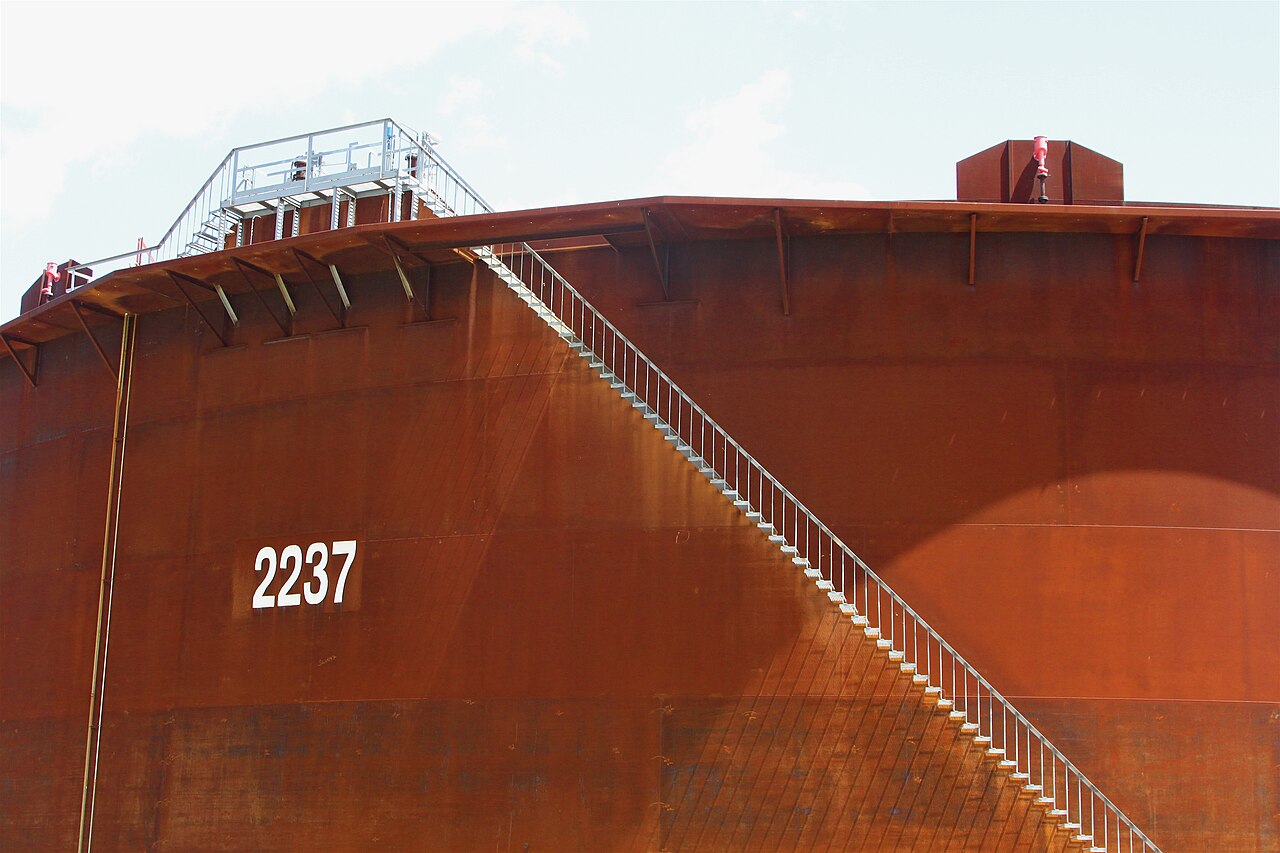
If supply and demand are the game, inventories are the scoreboard, and they are the single most useful fundamental series a trader can watch. Commercial stocks – refinery tanks, hubs, pipelines, ships – exist to buffer mismatches, so their direction of travel is the cleanest available reading of the balance: sustained builds mean supply exceeds demand, sustained draws mean the opposite. Level matters too, always measured against seasonal norms: the market convention is to compare against the five-year average for the same week, since raw levels mislead across seasons.
Within the US data, Cushing deserves special attention. It is the delivery point for the NYMEX WTI contract – roughly 90 million barrels of nameplate tankage in Oklahoma, fed and drained by pipelines like Basin and Keystone inbound and Seaway and other Gulf-bound lines outbound. Because futures converge on physical conditions at that specific hub, Cushing stocks move WTI spreads more directly than national totals do; the tank-tops scare of April 2020 and the tank-bottoms squeezes of 2023 both played out first in Cushing data. Why a landlocked Oklahoma tank farm anchors a global benchmark is a story of its own – covered in our guide to crude oil benchmarks.
Floating Storage and the Data You Cannot See
Onshore tank data covers the OECD well and the rest of the world poorly, which is why the market increasingly watches oil at sea. Satellite and transponder tracking of tankers turns floating storage – crude sitting on stationary, laden ships – into a global inventory proxy. Rising floating storage is one of the most reliable glut tells there is, because nobody pays tanker day-rates to store crude unless onshore tanks are full or the contango pays for it; in mid-2020 well over a hundred million barrels sat on the water. Draws in floating storage, conversely, often lead onshore draws by weeks. Most retail traders never look at it, which is exactly why it is worth the look.
The Futures Curve: Where the Balance Is Published
You do not need a subscription dataset to read the balance – the futures strip publishes it. When inventories are building and storage is filling, near-term contracts trade at a discount to deferred ones: contango. (The strip is public – the full forward curve for NYMEX WTI, 1,000 barrels per contract, is quoted years out.) The discount exists because someone has to be paid to hold the surplus; the spread covers tank rent and financing. When inventories are drawing and prompt barrels are scarce, near months trade over deferred: backwardation, the market paying a premium for oil now.
Keep the mapping straight, because getting it backwards inverts every signal: builds and glut go with contango; draws and tightness go with backwardation. The April 2020 super-contango – twelve-month WTI spreads beyond $10 – screamed glut, and made buying crude to store on chartered tankers a riskless-looking arbitrage. The steep backwardation of 2022 screamed scarcity. Watching the front spread day to day is like watching the balance in real time, which is why professionals often express fundamental views in calendar spreads rather than flat price; the mechanics of doing so are covered in our guide to how to trade crude oil futures.
Supply Shocks and the Risk Premium
Because demand cannot flex, sudden supply losses produce outsized price responses. The historical catalogue every analyst should know:
- 1973 Arab embargo: several million barrels a day withdrawn; prices roughly quadrupled in months.
- 1979-80 Iranian revolution, then the Iran-Iraq war: Iranian exports collapsed and prices more than doubled toward $40 – even though the net global supply loss was far smaller than the gross Iranian outage, panic buying and stockpiling amplified it.
- 1990 invasion of Kuwait: ~4 mb/d offline; prices doubled, then round-tripped within months once Saudi spare capacity filled the gap – the classic demonstration that outages plus spare capacity equal spikes that fade.
- 2019 Abqaiq attack: half of Saudi processing hit; the largest single-day percentage jump in Brent’s history, mostly retraced within weeks as repairs outran fears.
- 2022 Russia-Ukraine: feared loss of millions of barrels; Brent above $120. The barrels mostly kept flowing, rerouted at a discount, and price faded as that became clear.
The pattern: the market prices the feared loss immediately, then converges to the realized loss. That gap is the geopolitical risk premium, and it is mean-reverting. When tension headlines add $10 to crude and the tankers keep loading – as during the 2026 Hormuz scare, when roughly a fifth of world supply transits that strait and none of it actually stopped – the premium decays week by week. Fading fear is a legitimate strategy; just size it knowing that occasionally the feared barrels really do disappear.
EIA Wednesdays: Trading the Weekly Data

The highest-frequency fundamental input is the EIA Weekly Petroleum Status Report, published Wednesdays at 10:30 a.m. Eastern (the API’s survey lands the prior evening as a preview). The market reads five lines within seconds: the national crude build or draw versus consensus, the Cushing number, refinery utilization, gasoline and distillate stocks, and implied product demand. Prices react to the surprise, not the level – a 2-million-barrel build against a consensus draw is bearish; a 5-million-barrel build against a 7-million consensus is, perversely, bullish.
An honest word about trading it: most retail traders lose money on EIA releases, and the reasons are structural. The first print is traded by algorithms in milliseconds, so you are never first. The headline routinely conflicts with the internals – a big crude build caused by refinery maintenance says nothing bearish about demand, and the initial move often reverses once the details are parsed. And single weeks are noisy: import timing, ship schedules and adjustment factors swing the number by millions of barrels for reasons with no signal content. The professional approach is to trade the trend of four-to-six-week averages, use release-day volatility for entries rather than direction, and always read the report’s internals before believing its headline.
Forward Balances: The Three Forecasts That Frame the Market
Three agencies publish monthly supply-demand balances the whole market argues about: the IEA’s Oil Market Report, OPEC’s MOMR, and the EIA’s Short-Term Energy Outlook. Each projects demand growth, non-OPEC supply and the implied inventory change several quarters out. The forecasts disagree systematically – OPEC has tended to sit at the bullish end of demand estimates and the IEA at the transition-minded end, with spreads between them at times exceeding 1 mb/d – and the disagreement is itself information. When all three point the same direction, the market usually already trades there; the opportunity lives where you have a defensible reason to think one camp is wrong. Comparing current inventory trajectories against these projected balances is the cleanest way to build a view months ahead rather than reacting week to week.
A Worked Example: From Balance to Position
Concretely, suppose the next two quarters shape up like this: demand estimated at 104.5 mb/d on seasonal strength; non-OPEC supply at 70.5 mb/d; OPEC+ signaling output that implies 33.5 mb/d. That balance is short 0.5 mb/d – a draw of roughly 45 million barrels per quarter, about 1.5 percent of OECD commercial stocks each quarter. Historically, deficits of that size have supported firming backwardation and grinding price strength, so the analysis argues for long exposure – ideally partly in calendar spreads, which pay off if the draws materialize even when flat price gets pushed around by the dollar or equity risk appetite.
Now stress it. If OPEC+ compliance slips 20 percent, the deficit halves. If demand comes in 0.5 mb/d light on weaker Chinese buying, the deficit vanishes entirely. That sensitivity is the real lesson: oil balances live and die on half-million-barrel assumptions, which is why position sizing matters more than conviction, and why the weekly inventory data exists to tell you – promptly and impartially – whether your balance is wrong.
Turning Balances into Trades
How this framework cashes out in practice:
- Directional positions follow the projected balance: deficits ahead argue long, surpluses argue short – entered with technical timing, because fundamentals say nothing about the next 48 hours.
- Calendar spreads express inventory views cleanly. Expect builds, and you want to be short the front against the back (a bear spread), profiting as contango deepens. Expect draws, take the opposite side and let backwardation pay you. Spreads strip out much of the macro noise that whips flat price around.
- Seasonal trades exploit the calendar: gasoline strength into summer driving, distillate pull into winter, crude builds during spring refinery maintenance. These patterns are well known, which means they are partially priced – the edge is in years when positioning has crowded the wrong way.
- Risk-premium fades sell fear when the premium over your fundamental fair value gets stretched and physical flows remain undisturbed.
One overlay on all four: positioning. The CFTC’s weekly Commitments of Traders report shows how crowded the speculative side already is. A bullish balance that every managed-money account has already bought is a fragile trade – stretched net-length turns modest bearish surprises into cascades of liquidation. The strongest setups pair a fundamental view with positioning leaning the other way; the weakest pair consensus fundamentals with consensus positioning and call it conviction.
It is worth studying how the same framework behaves in a different commodity: natural gas runs on the identical inventory logic with far more brutal seasonality, and the contrast in our guide to natural gas supply and demand sharpens both analyses.
Common Mistakes in Fundamental Oil Analysis
- Trading fundamentals on a trading-day horizon. Balances play out over weeks and months; using them to predict tomorrow is astrology with spreadsheets.
- Treating US data as global data. The EIA series are the best in the world, but the US is a fifth of demand. A US draw during a global build is noise; Chinese imports and OECD totals complete the picture.
- Getting the curve backwards. Builds mean contango, draws mean backwardation. Plenty of published commentary still inverts this; check the logic, not the byline.
- Ignoring the “miscellaneous to balance” line. Every agency’s balance includes a residual that can exceed 1 mb/d. When your deficit is smaller than the residual, you do not have a deficit – you have an opinion.
- Anchoring on old regimes. Cost curves, OPEC strategy and demand trends all drift. The analyst who nailed 2011 was wrong for most of the following decade using the same numbers.
The Balance Sheet Habit
Strip away the noise and fundamental analysis is one discipline, repeated: keep a running global balance – supply by source, demand by region, the implied build or draw – and check it weekly against inventories and the shape of the curve. When your balance and the market’s price disagree, one of you is wrong, and finding out which is the job. Do that for a few quarters and OPEC headlines, EIA surprises and risk-premium spikes stop feeling like chaos and start feeling like moves on a board you already know. For how this fits alongside execution, risk management and the rest of the toolkit, go back to our complete guide to crude oil trading.